Manifold Learning [unfinished]
I. What is manifold learning
Dimensionality Reduction
- The accuracy of the training algorithms is directly proportional to the amount of data we have. However, managing a large number of features is usually a burden to our algorithm.
- Some of these features may be irrelevant, so it's important to make sure that the final model doesn't get affected by this.
- What is Dimensionality?
- Dimensionality refers to the minimum number of coordinates needed to specify any point within a space or an object.
- Why do we need Dimensionality Reduction?
- If you keep the dimensionality high, it will be nice and unique but it may not be easy to analyse because of complexity involved.
- Apart from simplifying data, visualization is also an interesting and challenging application.
Linear Dimensionality Reduction
- Principle Component Analysis
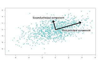
- Given a data set, PCA finds the directions along which the data has maximum variance in addition to the relative importance of these directions
- Example: Suppose that we feed a set of three-dimensional points that all lie on a two-dimensional plane to PCA. PCA will return two vectors that span the plane along with a third vector that is orthogonal to the plane. The two vectors that span the plane will be given a positive weight, but the third vector will have a weight of zero, since the data does not vary along that direction.
- PCA is most useful in the case when data lies on or close to a linear sub-space of the data set.
- More discussion on PCA can be found here: wiki or here.
Fig 1: PCA illustration (source: http://evelinag.com/blog)
What is manifold learning?
- What is manifold?
- You can think of it as a surface of any shape. It doesn’t necessarily have to be a plane i.e. it can be shaped like a folded sheet with all the curves.
Fig 2: data points are distributed in the shape of swiss roll
(source: what-is-manifold-learning )
- What is manifold learning?
- The manifold learning algorithms can be viewed as the non-linear version of PCA.
- If you think about approaches like PCA, you will realize that we are projecting the data onto some low-dimensional surface. But this is restrictive in the sense that those surfaces are all linear.
- Manifold learning comes with the assumption that the best representation lies in some weirdly shaped surface?
- How do we visualize it?
- The assumption is that the data points are actually samples from a low-dimensional manifold that is embedded in a high-dimensional space.
- Although the data points may consist of thousands of features, they may be described as a function of only a few underlying parameters.
- There are a lot of approaches to solve this problem such as Isomap, Locally Linear Embedding, etc. I will introduce some in the second part.
II. Some manifold learning algorithms
- Isomap
- Isomap can be viewed as an extension of Multi-dimensional Scaling (MDS).
- Isomap seeks a lower-dimensional embedding which maintains geodesic distances between all points.
- [24/10/2015] This link explains the graph-based technique to approximate the geodesic distances from the input matrix ( i.e. dissimilarity matrix).
- Locally Linear Embedding
- Locally linear embedding (LLE) seeks a lower-dimensional projection of the data which preserves distances within local neighborhoods.
- [31/10/2015] Here is detailed explanation for LLE.
- [31/10/2015] Pseudo code and illustration can be found here.
- Multi-dimensional Scaling
- Metric MDS
- Metric MDS tries to preserve the absolute pairwise distance.
- Non-metric MDS (NMDS)
- Non metric MDS focuses on the ordination of the data.
- t-distributed Stochastic Neighbor Embedding (t-SNE)
- t-SNE (TSNE) converts affinities of data points to probabilities. The affinities in the original space are represented by Gaussian joint probabilities and the affinities in the embedded space are represented by Student’s t-distributions.
- The Kullback-Leibler (KL) divergence of the joint probabilities in the original space and the embedded space will be minimized by gradient descent.
- Isomap can be viewed as an extension of Multi-dimensional Scaling (MDS).
- Isomap seeks a lower-dimensional embedding which maintains geodesic distances between all points.
- [24/10/2015] This link explains the graph-based technique to approximate the geodesic distances from the input matrix ( i.e. dissimilarity matrix).
- Locally linear embedding (LLE) seeks a lower-dimensional projection of the data which preserves distances within local neighborhoods.
- [31/10/2015] Here is detailed explanation for LLE.
- [31/10/2015] Pseudo code and illustration can be found here.
- Metric MDS
- Metric MDS tries to preserve the absolute pairwise distance.
- Non-metric MDS (NMDS)
- Non metric MDS focuses on the ordination of the data.
- t-SNE (TSNE) converts affinities of data points to probabilities. The affinities in the original space are represented by Gaussian joint probabilities and the affinities in the embedded space are represented by Student’s t-distributions.
- The Kullback-Leibler (KL) divergence of the joint probabilities in the original space and the embedded space will be minimized by gradient descent.


t-SNE is considered the state-of-the-art embedding algorithm.
ReplyDelete